🔗 Fluid Simulation Using Grid-Based Method
🔗 Background Fluid dynamics is a widely explored topic in natural sciences and has found extensive application in computer graphics, particularly in the simulation of fluid. In grid-based computational simulations, the Navier-Stokes equations are key to describing fluid dynamics in a natural and realistic manner. Joe Stam’s influential paper, “Stable Fluids” (1999), introduced a numerical solution for these equations, which has since become a foundational approach in computational fluid dynamics. While physically accurate fluid simulations are often complex and computationally expensive, our focus here is on solutions designed for game engines, prioritizing visual quality and real-time performance over strict physical accuracy. This approach allows for the creation of realistic effects, such as swirling smoke or fluid textures, with algorithms that remain stable and fast even with large time steps. In this blog post, we will explore how these algorithms can be implemented in 2D fluid simulations, offering both a theoretical understanding of the Navier-Stokes equations and practical insights into real-time applications.
🔗 Definitions
- Navier-Stokes Equations: These equations describe the balance of momentum for Newtonian fluids while incorporating the conservation of mass. They capture how fluid movement within a given domain is influenced by factors such as pressure, temperature, and density, all governed by Newton's second law of motion.
 Figure 1 : Navier-Stokes Equations
- Curl & Divergence: Divergence measures how much a fluid flows either into or out of a specific point in a vector field. On the other hand, curl quantifies the rotation or swirling motion of the fluid around a point, indicating how much it spins in the flow.
 Figure 2 : Curls & Divergence
- Lagrangian & Eulerian Viewpoints: The Lagrangian perspective tracks individual fluid particles as they move through space over time, whereas the Eulerian viewpoint focuses on observing changes in the velocity field within a fixed region of space. While the Lagrangian approach is often easier to understand conceptually, the Eulerian method simplifies the calculation of spatial derivatives.
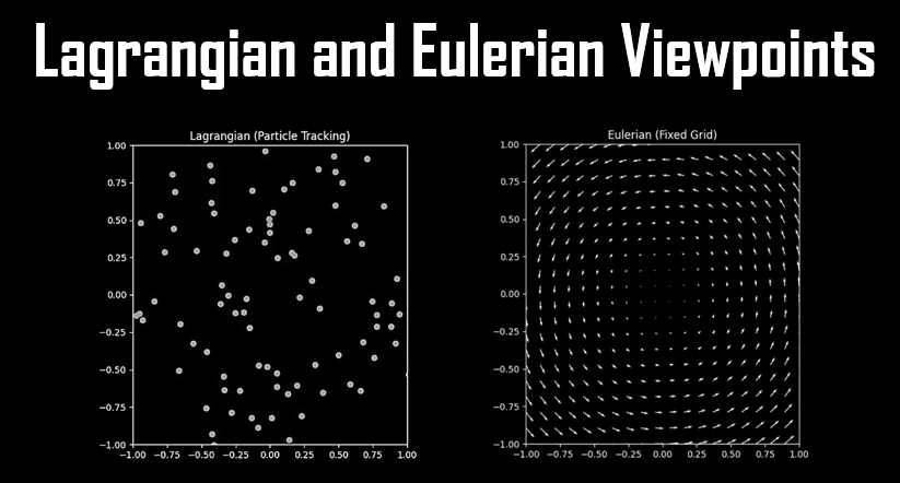 Figure 3 : Lagrangian & Eulerian Viewpoints
🔗 Fluid Forces Dynamics
 Figure 4 : Fluid Force Dynamics - Basic structure of the Fluid Force Dynamics where for each timestep it compute the three steps
Figure 1 : Navier-Stokes Equations
Figure 2 : Curls & Divergence
Figure 3 : Lagrangian & Eulerian Viewpoints
Figure 4 : Fluid Force Dynamics - Basic structure of the Fluid Force Dynamics where for each timestep it compute the three steps
- Initialize Grid Values: Begin by setting the initial values for each grid cell, defining the fluid's initial state across the simulation domain.
- Grid Value Modifiers: Adjust key variables based on user input or predefined settings, such as those controlled by a graphical user interface (GUI), to influence the simulation’s behavior.
- Viscous diffusion Compute the diffusion process to simulate how the fluid spreads out over time, accounting for the viscosity, which determines the fluid's resistance to flow and internal friction.
- Advection Calculate the movement of fluid particles within the grid, ensuring that fluid properties like velocity and temperature are transported accurately through the simulation space.
🔗 Force Dynamics Implementation
- Grid Initialization:
In this step, you define the initial state of the simulation by initializing key variables for each grid cell. These variables include color, depth, and velocity, as well as any additional variables that can enhance the visualization of fluid flow. This setup ensures a clear depiction of the fluid's starting state and provides a basis for observing how the fluid evolves over time.
- Grid Value Modification:
Dynamic modification of grid values is facilitated through various tools and interfaces. A common method is using a graphical user interface (GUI) to adjust parameters like velocity, pressure, and external forces. This allows for the simulation of environmental factors such as wind or gravity, interactions with solid objects, and adjustments for turbulence or boundary conditions. Real-time manipulation of these variables enhances the interactivity and customization of the simulation experience.
- Fluid Viscosity Diffusion:
Diffusion in fluid simulation spreads values like density or temperature to neighboring grid cells over time. Two main methods are used:
- Sum of Absolute Differences (SAD): This approach uses a linear relationship to calculate differences between a cell and its neighbors, applying a diffusion factor to spread values. Although straightforward, SAD can cause instability with large diffusion rates, leading to oscillations and divergence.
- Smooth Diffusion: Based on Joe Stam's technique, this method finds future values that, when reversed in time, match the current state. This hyperbolic relationship ensures stability, avoiding oscillations and divergence, but introduces the challenge of solving a linear system of unknowns.
- Advection Step:
Advection describes how quantities like smoke or fluid density move based on velocity. The reverse advection technique traces values backward in time to their original positions, using the inverted velocity field. This method maintains stability and ensures smooth transitions. After computing new positions, values are interpolated across neighboring cells using bilinear interpolation to ensure a smooth distribution.
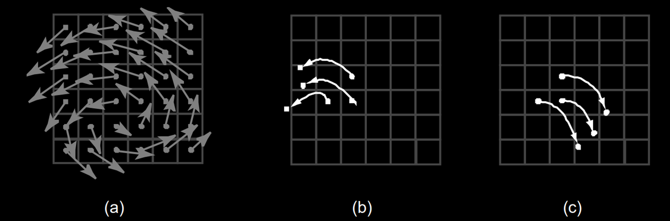 Figure 5 : Forward Advection & Backtrace Advection : Basic idea behind the advection step. Instead of moving the cell centers forward in
time (b) through the velocity field shown in (a), we look for the particles which end up exactly at
the cell centers by tracing backwards in time from the cell centers (c).
Figure 5 : Forward Advection & Backtrace Advection : Basic idea behind the advection step. Instead of moving the cell centers forward in
time (b) through the velocity field shown in (a), we look for the particles which end up exactly at
the cell centers by tracing backwards in time from the cell centers (c).
🔗 Domain Behavior
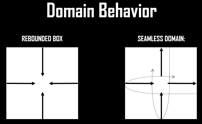 Figure 6 : Domain Behavior; Rebound Domain & Seamless Domain
- Grid Initialization:
In this step, you define the initial state of the simulation by initializing key variables for each grid cell. These variables include color, depth, and velocity, as well as any additional variables that can enhance the visualization of fluid flow. This setup ensures a clear depiction of the fluid's starting state and provides a basis for observing how the fluid evolves over time.
- Grid Value Modification:
Dynamic modification of grid values is facilitated through various tools and interfaces. A common method is using a graphical user interface (GUI) to adjust parameters like velocity, pressure, and external forces. This allows for the simulation of environmental factors such as wind or gravity, interactions with solid objects, and adjustments for turbulence or boundary conditions. Real-time manipulation of these variables enhances the interactivity and customization of the simulation experience.
- Fluid Viscosity Diffusion:
Diffusion in fluid simulation spreads values like density or temperature to neighboring grid cells over time. Two main methods are used:
- Sum of Absolute Differences (SAD): This approach uses a linear relationship to calculate differences between a cell and its neighbors, applying a diffusion factor to spread values. Although straightforward, SAD can cause instability with large diffusion rates, leading to oscillations and divergence.
- Smooth Diffusion: Based on Joe Stam's technique, this method finds future values that, when reversed in time, match the current state. This hyperbolic relationship ensures stability, avoiding oscillations and divergence, but introduces the challenge of solving a linear system of unknowns.
- Advection Step:
Advection describes how quantities like smoke or fluid density move based on velocity. The reverse advection technique traces values backward in time to their original positions, using the inverted velocity field. This method maintains stability and ensures smooth transitions. After computing new positions, values are interpolated across neighboring cells using bilinear interpolation to ensure a smooth distribution.
Figure 5 : Forward Advection & Backtrace Advection : Basic idea behind the advection step. Instead of moving the cell centers forward in
time (b) through the velocity field shown in (a), we look for the particles which end up exactly at
the cell centers by tracing backwards in time from the cell centers (c).
Figure 6 : Domain Behavior; Rebound Domain & Seamless Domain
Rebound domain behavior suggests a domain where the fluid hits the boundaries and is reflected back into the domain, as if the walls act like mirrors to the flow and this is what i used for my project. While Seamless Domain behavior indicates a continuous flow, where the fluid leaving one side of the domain immediately re-enters from the opposite side, creating a seamless loop.
🔗 Projection
The projection step ensures that the fluid remains mass-conserving and incompressible, which is crucial for accurately simulating fluid dynamics using the Navier-Stokes equations. To achieve this, the velocity field must be corrected, as it typically doesn't conserve mass after earlier steps. Simply solving the underlying partial differential equations can lead to instability, so numerical stability is vital for the simulation to produce reliable results. This is where the Helmholtz-Hodge decomposition comes in, which allows us to split the velocity field into two components: a mass-conserving field with desired vortex-like patterns and a gradient field, which causes unwanted inward or outward flows. By subtracting the gradient field from the velocity field, we correct it to be mass-conserving. This correction involves solving a linear system called the Poisson equation, stabilizing the simulation and ensuring the fluid behaves realistically.
 Figure 7 : Helmholtz-Hodge decomposition
🔗 Simulation and Visualization
The fluid simulation procedure begins by initializing key variables, such as velocity and density fields. While the simulation is active, the previous timesteps for both velocity and density are retained. The velocity field is then computed using fluid forces such as external forces, diffusion, and advection, followed by the computation of the density field using similar dynamics. Finally, a projection step is performed to ensure mass conservation, after which the simulation results are visualized. This process is repeated continuously for each simulation step.
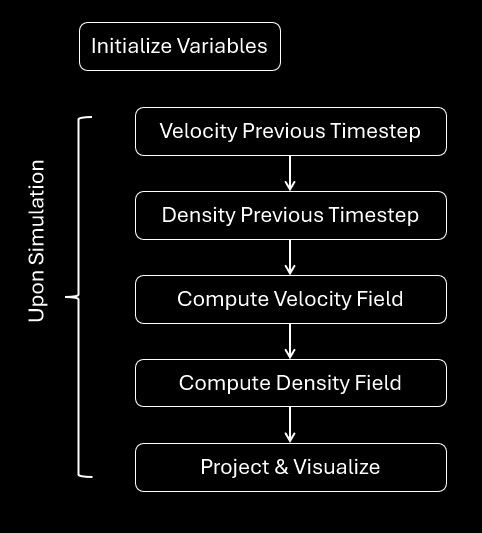 Figure 8 : Simulation steps
🔗 Output

Bashar Beshoti
I'm a a Computer Science student and an avid junior software developer with a passion for a variety of subjects, including computer graphics, computer vision, image processing, and software engineering. Additionally, I have a side hobby and minor interest in animation and sound creation.